TinyML on MCU: from dataset to real-time inference in Rust firmware
🟠 In this article, I walk through the complete TinyML lifecycle on a microcontroller — from dataset preparation and model training to running TensorFlow Lite Micro on bare metal and integrating the model into a Rust firmware via a custom FFI wrapper.
This project intentionally spans multiple domains: embedded systems, machine learning, data engineering, and low-level systems programming in Rust.
Defining the task and the TinyML pipeline
The goal of the project is to deploy a binary classifier that determines whether a person is present in front of a camera — entirely on-device, without cloud inference.
This kind of TinyML project forces you to reason about the full ML lifecycle, not just training accuracy. The resulting pipeline looks like this:
- Collecting, cleaning, and labeling raw image data
- Designing data augmentations for robustness
- Writing Python scripts for preprocessing and training
- Validating models and selecting an optimal architecture
- Quantizing the model and converting
.keras → .tflite - Evaluating KPIs before and after quantization
- Embedding the model into MCU firmware
- Building a safe wrapper and running inference on-device
- Optimizing memory usage (arena sizing, cache alignment)
Dataset preparation: from camera frames to folders
High-quality labeled data is the single most important factor in supervised learning.
A model trained on weak or biased data will fail silently, especially on-device where debugging is expensive.
For this project:
- The original dataset is split into train and test
- A validation subset is derived from the training data
- Training and validation sets are used for optimization and tuning
- The test set is kept strictly isolated for evaluation
Because a representative dataset without bias requires careful balancing across age, gender, ethnicity, lighting conditions, and backgrounds, I combined:
- large open-licensed face datasets;
- additional frames captured directly from the target device.
The not_person class is intentionally broad: any image without a human face qualifies.
All images were:
- resized to 160×120;
- converted to grayscale;
- labeled and class-balanced.
dataset/
 ├── test/
 │    ├── no_person/ 1726 images
 │    └── person/    1726 images
 ├── train/
 │    ├── no_person/ 11740 images
 │    └── person/    11740 images
 └── val/
      ├── no_person/ 3666 images
      └── person/    3666 images
Data augmentation pipeline
To ensure the model generalizes to real-world conditions, the dataset is passed through an augmentation pipeline during training.
The goal is not to artificially inflate the dataset, but to expose the model to:
- rotations and framing variance;
- brightness changes;
- scale distortions;
- mirrored perspectives.
A typical augmentation block looks like this:
data_augmentation = keras.Sequential(
    [
        layers.Rescaling(1.0 / 255, dtype="float32"),
        layers.RandomFlip("horizontal"),
        layers.RandomRotation(0.08),
        layers.RandomZoom(0.2),
        layers.RandomBrightness(0.1, value_range=(0.0, 0.6)),
    ]
)
Preprocessing is intentionally embedded inside the model graph — this becomes important later during quantization.
Model training strategy
The model must satisfy two constraints simultaneously:
- be accurate enough for real-world inference;
- be small and efficient enough to run on an MCU.
After experimentation, MobileNetV2 proved to be the best tradeoff for this task. The architecture was adapted to accept grayscale input.
Training was split into two distinct phases.
Head-only training
In the first phase:
- the MobileNetV2 backbone is fully frozen;
- only the classification head is trained;
- optimizer:
Adam(1e-3); - callbacks:
EarlyStopping,ReduceLROnPlateau,ModelCheckpoint.
This allows the classifier to adapt to the grayscale domain without destabilizing pretrained features.
Fine-tuning the backbone
After convergence:
- the top 60 layers of MobileNetV2 are unfrozen;
- these layers capture higher-level patterns that benefit from domain adaptation.
After fine-tuning, the model consistently reaches 92–96% accuracy on the test set, depending on noise and data distribution.
Evaluating the FP32 model
Before quantization, the .keras model is evaluated to establish a baseline.
For binary classification, the most informative visualization is the confusion matrix, which exposes class-specific failure modes.
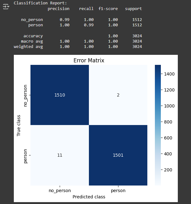
These FP32 results are later compared against the INT8 version to measure acceptable degradation. Once the baseline met expectations, I moved on to model compression.
INT8 quantization for MCU deployment
Quantizing the model to INT8:
- reduces model size by approximately 4×;
- enables efficient execution on MCU-class hardware;
- eliminates floating-point dependencies.
The conversion requires a custom wrapper that:
- defines correct
uint8/int8input and output behavior; - ensures preprocessing (e.g. division by 255) is part of the graph;
- guarantees that all internal ops remain INT8-compatible.
If unsupported operations remain, TensorFlow will insert float fallbacks — and such a model will not run on TensorFlow Lite Micro.
Post-quantization TFLite evaluation
Quantization inevitably reduces precision by collapsing FP32 weights into 8-bit integers. Before deploying to firmware, a sanity check is mandatory.
The INT8 .tflite model is loaded into a TFLite interpreter, and:
- random samples from the test set are evaluated;
- accuracy and confusion matrices are compared against the FP32 baseline.
As long as degradation stays within acceptable limits, the model is considered deployment-ready. At this point, the pipeline is ready to transition from Python to Rust firmware and on-device inference.